
FREE RESOURCE
How to Build a Dynamic Excel Dashboard That Updates Automatically automatically
Learn how to build an Excel dashboard that updates automatically as you add new data, with no pivot tables and no manual refresh. Includes a free downloadable template you can adapt to your own reporting.
How to Build a Dynamic Excel Dashboard That Updates Automatically
You update your data. The chart doesn't move. So you click Refresh, fix a range, or rebuild something that worked last week.
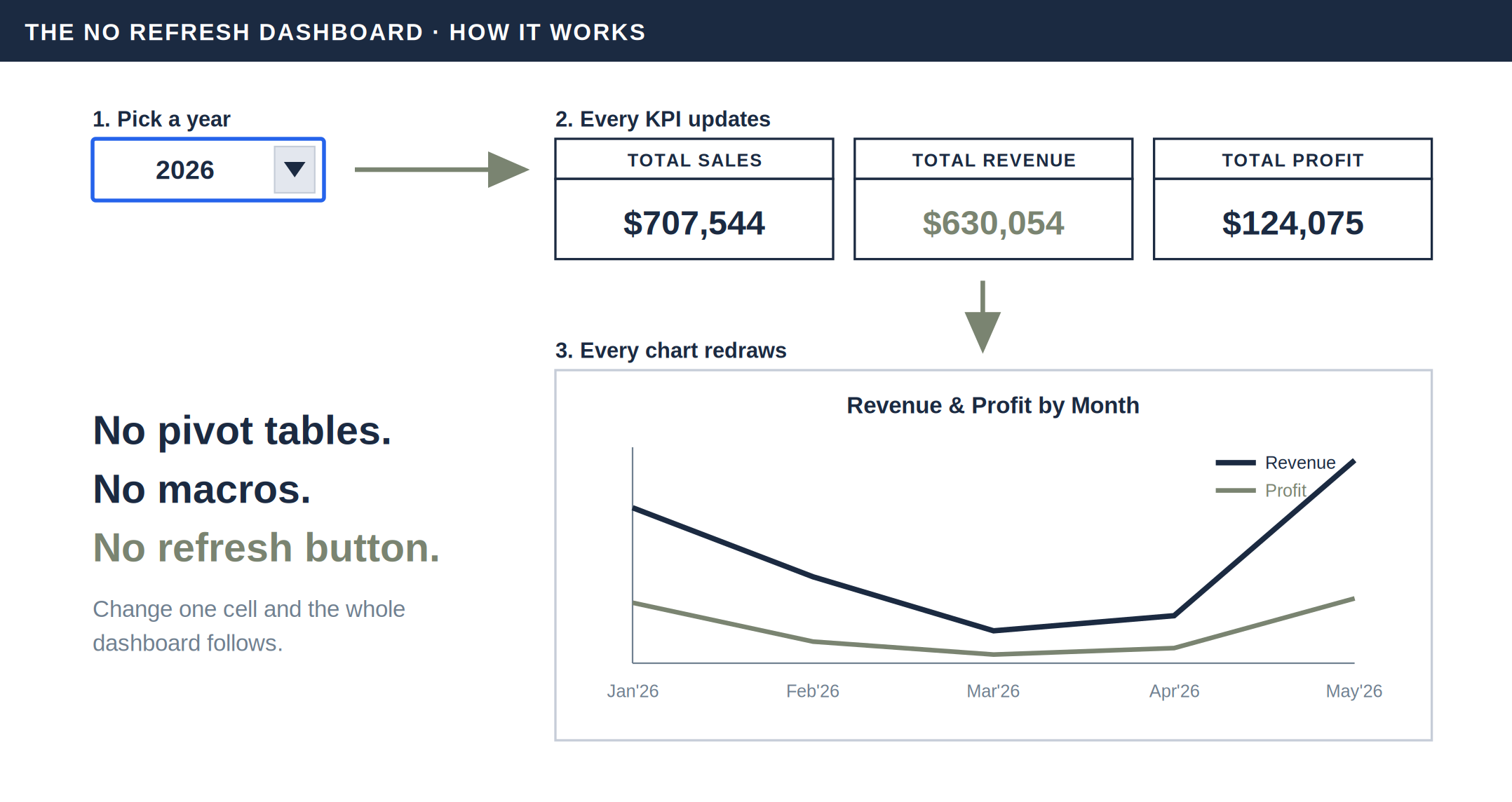
It doesn't have to work that way. With a dynamic Excel dashboard, you add new data and everything on the page updates by itself. No pivot tables, no refresh button, no macros, and no tools outside of Excel.
This is the exact setup we use at XINDARA for client reporting, explained in plain steps. There's also a free template at the bottom of this post with the whole thing already built, so you can follow along or skip straight to a working copy.
Why your dashboard breaks when you add new data
Most Excel dashboards point at fixed ranges. A formula like =SUM(B2:B50) only looks at rows 2 through 50. Add a row 51 and the formula never sees it. Your chart has the same problem. It's locked to the rows it was given when you built it.
Pivot tables help, but they hold a snapshot of your data and only update when you click Refresh. Someone always forgets.
The fix is to build with ranges that grow on their own. That's the whole trick, and Excel has had the tools for it since Excel 2021.
Building the dynamic Excel dashboard, step by step
Eight steps, each one small. If you have the free template open, you can see every step already wired up.
Step 1: Turn your data into an Excel Table
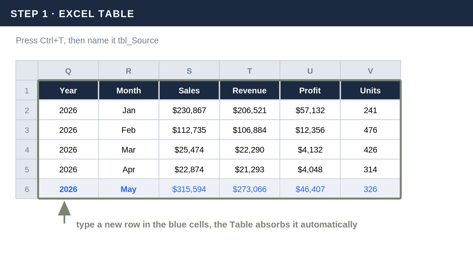
Click anywhere in your data and press Ctrl+T. Check "My table has headers." Then go to the Table Design tab and name it tbl_Source.
Tables are the foundation because they grow automatically. Type a new row under the last one and the Table absorbs it. Anything connected to the Table sees the new row instantly.
Step 2: Let Excel fill in the dates
Nobody should type "2026" and "Mar" by hand every time they add a row. In the template, the date columns calculate themselves: each row's Year Month is just the previous row's date plus one month, using EDATE(), and the Year and Month columns read from it. You type your numbers, the dates handle themselves.
Step 3: Add a Year dropdown
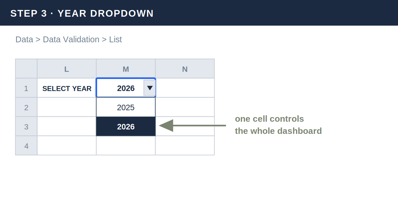
Pick one cell to control the whole dashboard. Select it, go to Data > Data Validation > List, and enter your years, like 2025, 2026.
This one cell is your dashboard's steering wheel. Everything you build next reads from it.
Step 4: Pull the selected year's data with FILTER
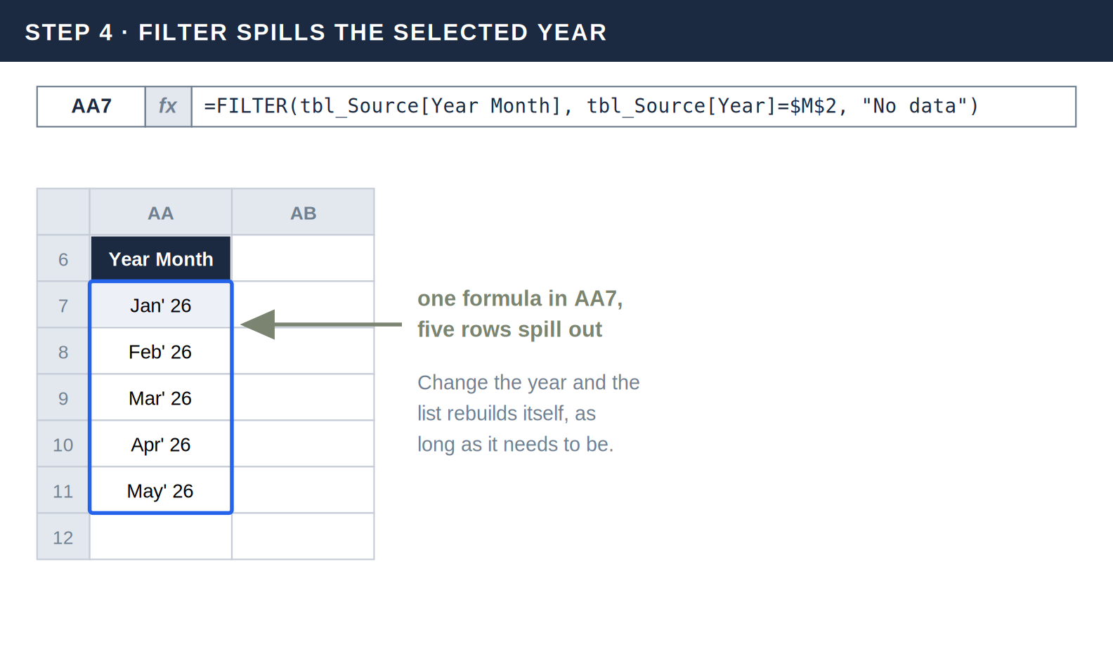
In an out-of-the-way column, write:
=FILTER(tbl_Source[Year Month], tbl_Source[Year]=$M$2, "No data")($M$2 is wherever you put your dropdown.) This one formula returns every month for the selected year, spilling down as many rows as it needs. Pick a different year in the dropdown and the list rebuilds itself. You write it once and never touch it again.
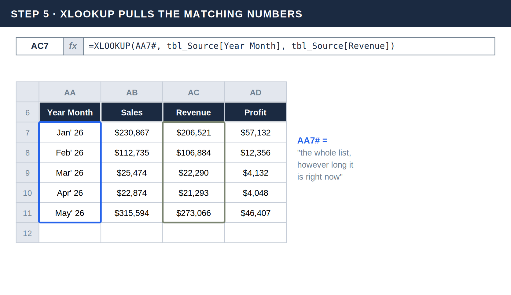
Step 5: Pull the matching numbers with XLOOKUP
Next to your month list, bring in the numbers for each month:
=XLOOKUP(AA7#, tbl_Source[Year Month], tbl_Source[Revenue])AA7 is the first cell of your FILTER list, and the # tells Excel "the whole list, however long it is right now." Repeat this formula for each column you want, like Sales, Profit, and Units. When the month list grows or shrinks, these columns follow automatically.
Step 6: Name your ranges
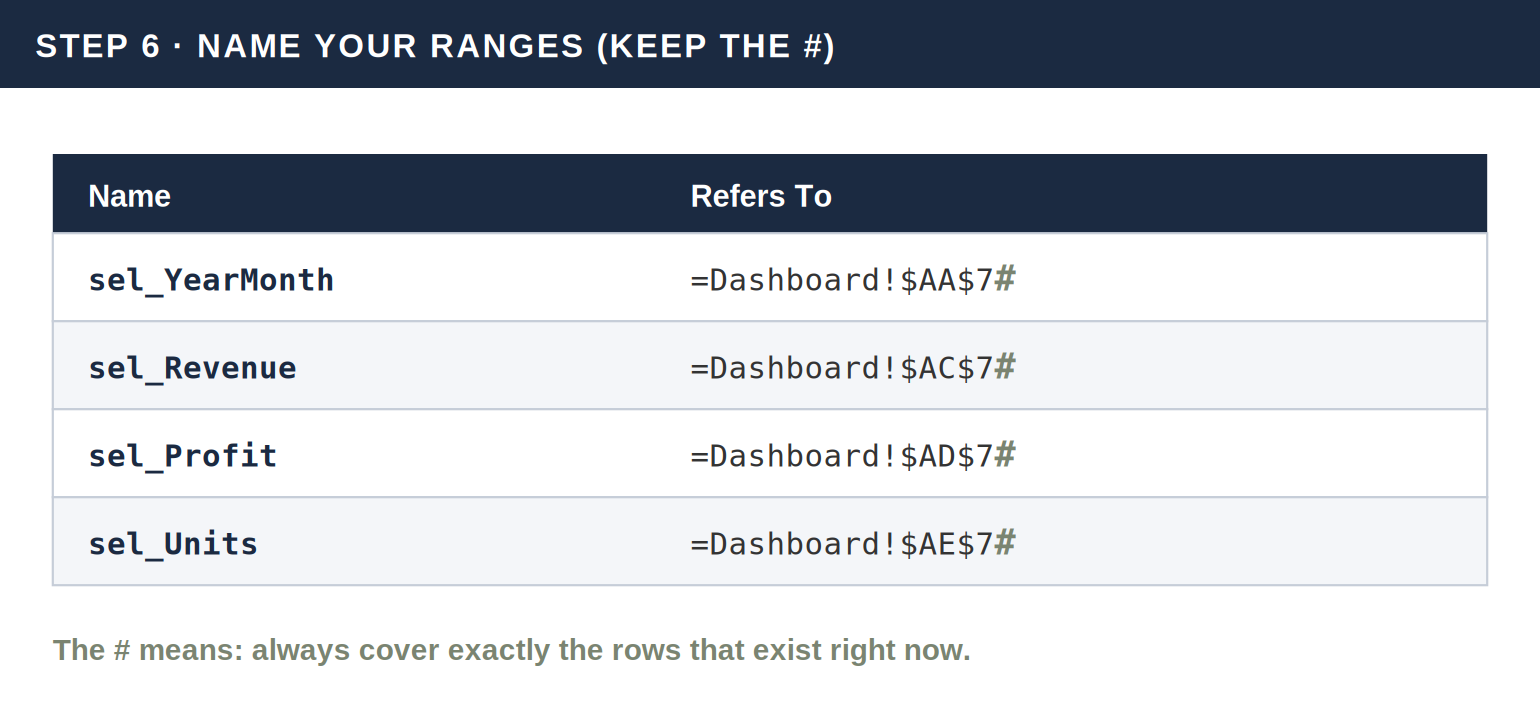
Go to Formulas > Name Manager and create a name for each column you just built, keeping the #:
sel_YearMonth=Dashboard!$AA$7#sel_Revenue=Dashboard!$AC$7#sel_Profit=Dashboard!$AD$7#sel_Units=Dashboard!$AE$7#
These names are what make the next two steps easy. Because of the #, each name always covers exactly the rows that exist right now.
Step 7: Point your KPI cards at the names
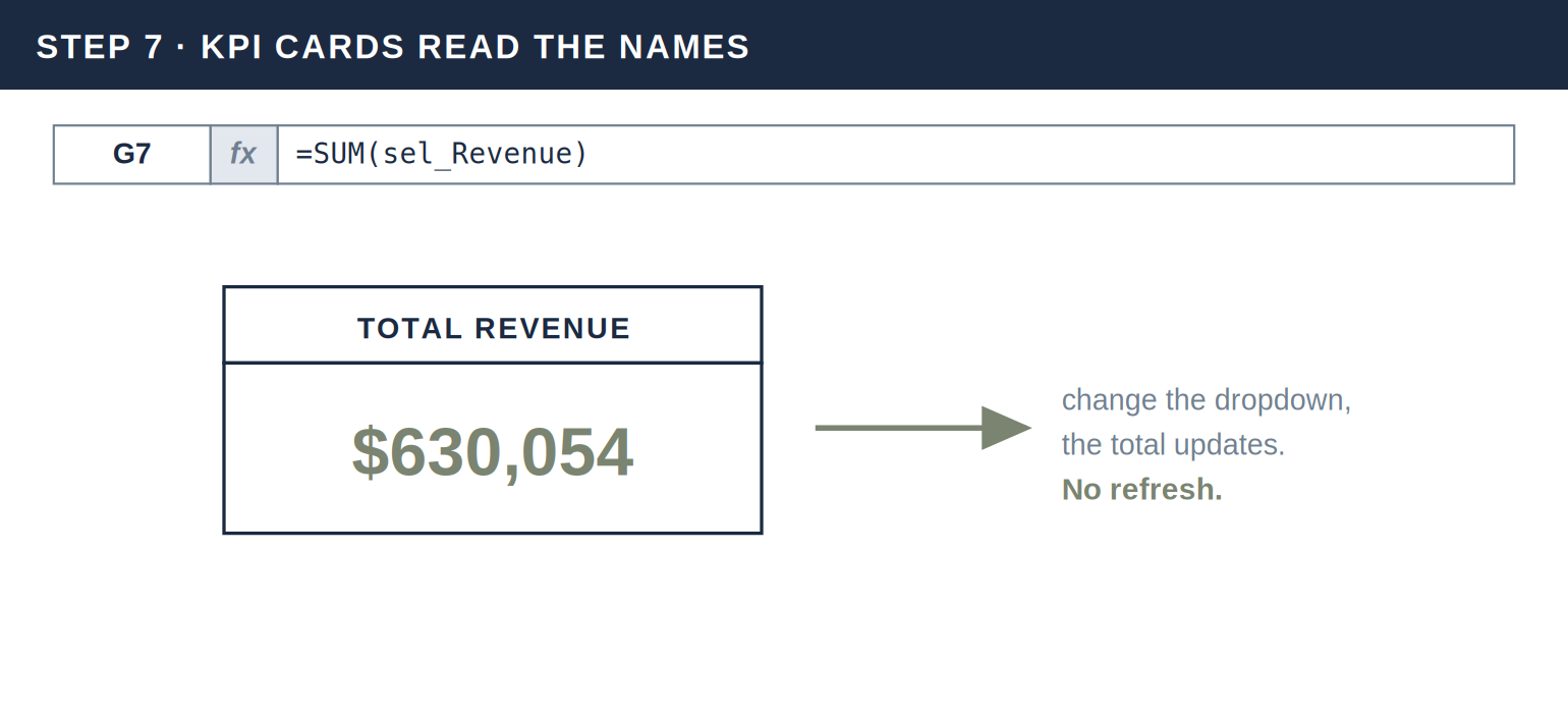
Your totals become one-line formulas:
=SUM(sel_Revenue)Change the year in the dropdown and watch the totals change with it. No refresh needed.
Step 8: Point your charts at the names too
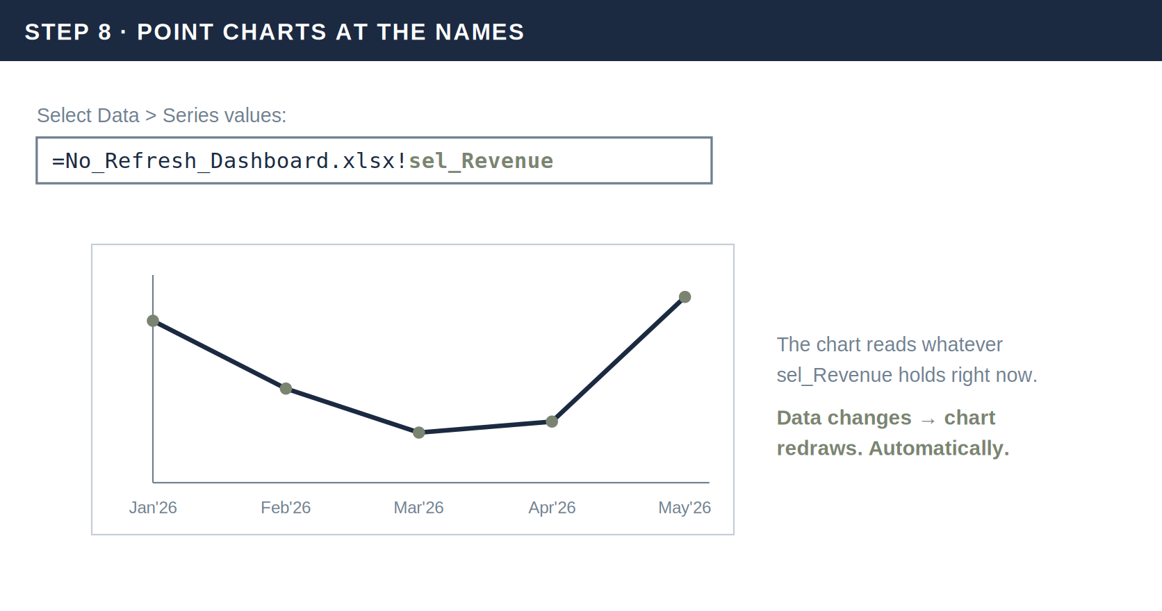
This is the step most tutorials skip. Right-click your chart, choose Select Data, and edit each series. Instead of a fixed range, type the workbook name plus the named range:
=YourWorkbookName.xlsx!sel_RevenueDo the same for the axis labels using sel_YearMonth. Your chart now reads from a range that resizes itself, which means it redraws the moment your data changes.
Why this never needs a refresh
Pivot tables keep a copy of your data and only update that copy when you ask. This setup keeps no copy. Every formula reads live from your Table, every time Excel recalculates, which is every time anything changes.
Change the dropdown, and the FILTER list rebuilds, the XLOOKUP columns follow, the named ranges resize, and every KPI and chart pointed at them updates. It's one chain reaction, and it runs itself.
Four things to know before you build
You need Excel 2021 or Microsoft 365. The # operator and FILTER don't exist in older versions.
Chart references need the workbook name. If you rename the file, update the chart references to match.
XLOOKUP grabs the first match only. If the same month appears on multiple rows, it won't add them together. The template's data is structured so this isn't an issue, and it's something to keep in mind with your own data.
Don't type over the date columns. They're formulas. Overwriting one breaks the chain below it.
The pattern, in one line
Table, FILTER, XLOOKUP, named ranges with #, charts pointed at the names. Each layer feeds the next, nothing is hardcoded, and the dashboard just works.
We build dynamic Excel dashboards this way at XINDARA because it meets people where they already work. No new software, no new skills for the team. They update their data and the dashboard keeps up.
Questions, or want help adapting this to something more complex like multiple regions or rolling 12-month views? Reach out at team@xindara.com.
Where accuracy matters most
that's where we work
We work anywhere documents carry risk, financial impact, or compliance requirements.





What you're probably
wondering
Quick answers to the most common questions
How do I make an Excel dashboard update automatically without a refresh?
Build it on ranges that resize themselves instead of fixed cell references. Start with an Excel Table to hold your data, since Tables absorb new rows automatically. Use FILTER to pull the slice you want and XLOOKUP to line up the matching numbers, then name those results with the # spill reference operator so the named range grows and shrinks with your data. Point your charts and KPI cards at those names instead of a fixed range, and the whole dashboard updates the moment your data changes. No Refresh button, no macros, no Pivot Tables. It works in Excel 2021 and Microsoft 365.
Why does my Excel chart not update when I add new data?
Your chart is pointed at a fixed range, so it only sees the rows it was given when you built it. A chart bound to B2:B50 will never pick up row 51, and a formula like SUM(B2:B50) has the same blind spot. Pivot tables get around this but hold a snapshot that only updates when someone clicks Refresh, which someone always forgets. The fix is to bind your chart to a named range built with the # spill operator instead of a fixed range, so it resizes with your data and redraws on its own every time anything changes.
Are Pivot Tables the only way to build a dynamic dashboard in Excel?
No. Pivot Tables are one option, but you can build a fully dynamic dashboard with no Pivot Tables, no macros, and no add-ins using dynamic array formulas. An Excel Table holds the data, FILTER and XLOOKUP pull and align the numbers, and named ranges built with the # spill reference operator keep everything sized to the current data. This approach reads live from your source every time Excel recalculates, so unlike a Pivot Table it never holds a stale snapshot and never needs a manual refresh. It's often lighter and easier for a team to maintain since there's nothing to rebuild or re-refresh.
What Excel version do I need for FILTER, XLOOKUP, and the # spill operator?
You need Excel 2021 or Microsoft 365. FILTER, XLOOKUP, and the # spill reference operator are all dynamic array features, and they don't exist in Excel 2019 or earlier. If your formulas return a #NAME? error, that's usually the sign you're on a version that doesn't support them. This applies to both Windows and Mac, and to the web version of Excel in a Microsoft 365 subscription. If your team is on an older version, upgrading to Microsoft 365 is the only way to use this approach, since there's no add-in that backports these functions.